

full
stack
360
agency


Award-winning Web Design London agency, we specialise in delivering creative and innovative solutions that encompass everything from website design and app development to software creation, AI integration, and digital transformation.
As an award-winning Web Design London agency, we excel in creative solutions ranging from website design and app development to AI integration and digital transformation.
We’re a full 360 service which means we’ve got you covered on idea, design, development right through to digital and social marketing. You’ll form a lasting relationship with us, collaboration is central to everything we do, think of us as an extension to your team. We’ll push you out of your comfort zone from time-to-time, but this is where you’ll shine, you’re in good hands.
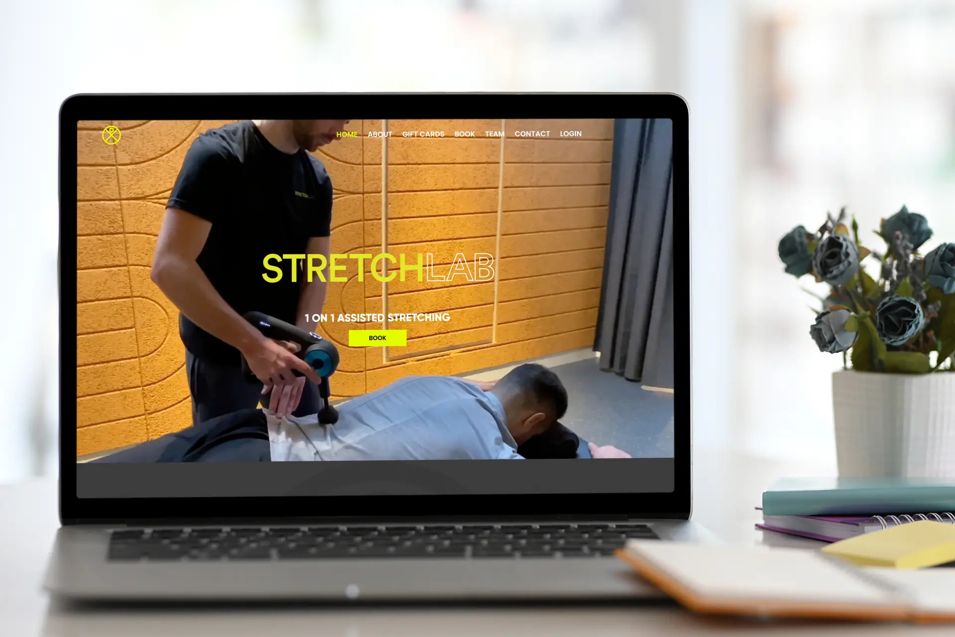
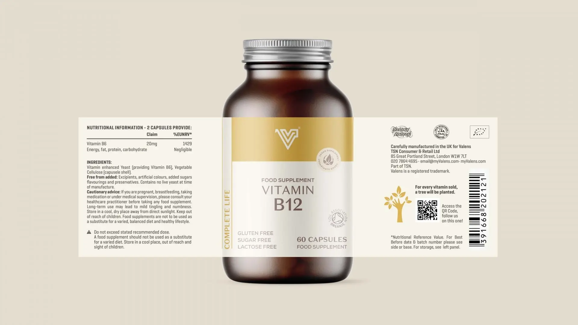
Some featured projects

We've worked with
some of the greats
Why the name?
So let’s address the burning question, why are you called Ikaroa? Pronounced i-ka-roa, in Māori mythology Ikaroa is the long fish that gave birth to all the stars in the Milky Way or the Mother Goddess of all the stars… that’s exactly what we do, we give birth to stars, we are there from the very start and will help nurture you and your idea every step of the way, we are the secret behind many global brands, celebs, start-ups and entrepreneurs, welcome to Ikaroa.
We've worked with
some of the greats

Creative studio with
art & technologies.
Forward-thinking team of designers and developers.
Strategy
Decades of experience between us, let’s talk, understand your idea and create a strategy together on how we can turn your vision into reality.
Create
Let’s create, from initial planning, sketching, wire-framing to full stack design, we will keep your vision in mind and create it.
Develop
Development is all about what you see under the hood, not just above, user experience is key and should be friction free.
Amplify
We market to millions of people everyday and know what works and what doesn’t – Delivering a strong return on investment is our priority, if we can achieve that, then we have both won. Social media is in our blood, we live it and breathe it and can help elevate your brand a cut above the rest.
Domains & Hosting
We have decades of experience and can help secure your new domain name, set up your website and set up your emails within minutes.
24/7 Support
Our domains & hosting team are on hand 24 hours a day, 7 days a week. If you need a new domain or need changes made to your server, we're here to help anytime.
Drop us a note and we'll be in touch
Email us
For project inquiries only:
[email protected]
For other questions:
[email protected]